Statistics in IB Math often starts deceptively simple. You might think, “I know how to find the average,” or “I can find the middle number.” But as any experienced IB student knows, the curriculum quickly shifts from basic arithmetic to complex logical reasoning. Suddenly, you aren’t just adding numbers; you are dealing with discrete versus continuous data, frequency tables, and “buckets” of data where the exact values are unknown.
Whether you are in AA or AI, Standard or Higher Level, understanding the measures of central tendency is the bedrock of your statistical knowledge. These measures—Mean, Median, and Mode—are not just formulas; they are the tools we use to summarize vast amounts of data into a single, representative value.
In this guide, we will move beyond the basics. We will explore how to handle large datasets efficiently using frequency tables, how to calculate the estimated mean for continuous data, and the specific algebraic formulas you need to find the median position without writing out hundreds of numbers. We will also cover the essential TI-Nspire calculator hacks (Menu 4.1.1) that can save you precious minutes during your exams.
The Three Pillars of Central Tendency
Before we dive into the complex calculations, we must ensure our definitions are airtight. In IB Math, definitions often carry subtle nuances that can lead to “trap” questions on exams.
1. The Mean (Arithmetic Average)
The mean is the most common measure of central tendency. It is calculated by summing all data points and dividing by the total number of points (n).
Mathematical notation for the mean of a sample is often denoted as \bar{x}:
\bar{x} = \frac{\sum_{i=1}^{n} x_i}{n}
While this is straightforward for a list of numbers, it becomes tricky when dealing with grouped data, which we will discuss later.
2. The Median ( The Middle Value)
The median is the value separating the higher half from the lower half of a data sample. It is the physical “middle” of your sorted data. The challenge with the median in IB Math isn’t identifying it in a list of five numbers; it is finding it in a list of 50 or 100 numbers without writing them all out.
3. The Mode (The Most Frequent)
The mode is the value that appears most frequently in a data set. There is a common misconception here regarding what happens when data points appear equally.
- One Mode: One number appears more than any other.
- Multi-modal: Multiple numbers tie for the highest frequency.
- No Mode: If all numbers appear the exact same amount of times (e.g., every number appears once, or every number appears twice), there is no mode. It is incorrect to say “all of them are the mode.”
Discrete vs. Continuous Data: Why It Matters
To choose the correct method for calculating central tendency, you first need to identify the type of data you are working with. The IB curriculum distinguishes strictly between discrete and continuous data.
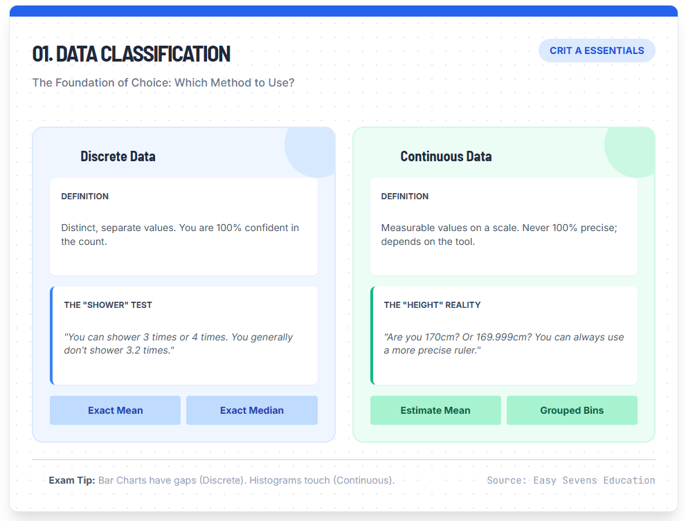
01. Data Classification
The Foundation of Choice: Which Method to Use?
Discrete Data
Definition
Distinct, separate values. You are 100% confident in the count.
The "Shower" Test
"You can shower 3 times or 4 times. You generally don't shower 3.2 times."
Continuous Data
Definition
Measurable values on a scale. Never 100% precise; depends on the tool.
The "Height" Reality
"Are you 170cm? Or 169.999cm? You can always use a more precise ruler."
Discrete Data
Discrete data consists of distinct, separate values. These are values you can count with 100% confidence.
“How many times did you shower this week? You can shower 3 times, 4 times, or 5 times. You generally don’t shower 3.2 times.”
Because these values are concrete, we can calculate an exact mean and an exact median.
Continuous Data
Continuous data represents measurements where you can never be 100% precise. Examples include height, weight, time, or temperature.
“If you measure your height as 170 cm, are you exactly 170? Or are you 170.1? Or 169.999? You can always use a more precise ruler to get more decimal places.”
Because continuous data is often grouped into intervals (or “buckets”) to make it manageable, we often cannot calculate an exact mean—we can only calculate an estimate mean.
Summary: Data Types and Calculation Strategy
| Feature | Discrete Data | Continuous Data |
|---|---|---|
| Definition | Countable, distinct values (e.g., number of apples, shoe size). | Measurable values on a scale (e.g., height, weight, speed). |
| Visual Representation | Bar Chart (bars separated). | Histogram (bars touching). |
| Mean Calculation | Exact calculation possible. | Estimate Mean using mid-interval values. |
| Grouping | Frequency Tables (Values). | Frequency Tables (Intervals/Buckets). |
How to Calculate Median Algebraically (The Position Method)
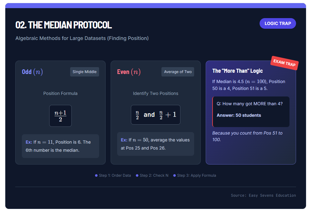
02. The Median Protocol
Algebraic Methods for Large Datasets (Finding Position)
Odd \( (n) \)
Single MiddlePosition Formula
Even \( (n) \)
Average of TwoIdentify Two Positions
The "More Than" Logic
If Median is 4.5 (\( n=100 \)), Position 50 is a 4, Position 51 is a 5.
Q: How many got MORE than 4?
Answer: 50 students
Because you count from Pos 51 to 100.
Imagine a dataset with 50 students. Writing out 50 numbers to find the middle is inefficient and prone to error. Instead, we use algebraic rules to find the position of the median, and then we identify the value at that position.
Step 1: Order the Data
Data must always be in ascending order (smallest to largest) before finding the median.
Step 2: Determine if n (Total Frequency) is Odd or Even
Case A: Odd Number of Data Points
If you have an odd number of values (e.g., n=11), there is exactly one middle number.
Formula for Position:
\text{Position} = \frac{n+1}{2}
Example: If n=11, the median is at position \frac{11+1}{2} = 6. The 6th number is your median.
Case B: Even Number of Data Points
If you have an even number of values (e.g., n=50), there is no single middle number. You must average the two middle values.
The Two Middle Positions are:
\frac{n}{2} \quad \text{and} \quad \frac{n}{2} + 1
Example: For 50 students (n=50):
- Position 1: 50 / 2 = 25
- Position 2: 25 + 1 = 26
The median is the average of the values at Position 25 and Position 26.
The “More Than” Trap
In logic questions, you may be asked: “How many students obtained a grade of more than 4?” given the median or quartiles.
If the median is 4.5 (meaning the middle lies between a 4 and a 5), and n=100:
- Position 50 is a 4.
- Position 51 is a 5.
Since the question asks for “more than 4,” you start counting from Position 51. From 51 to 100 is exactly 50 students. This type of logical deduction is a favorite in IB exams.
Handling Grouped Continuous Data (The “Bucket” Method)
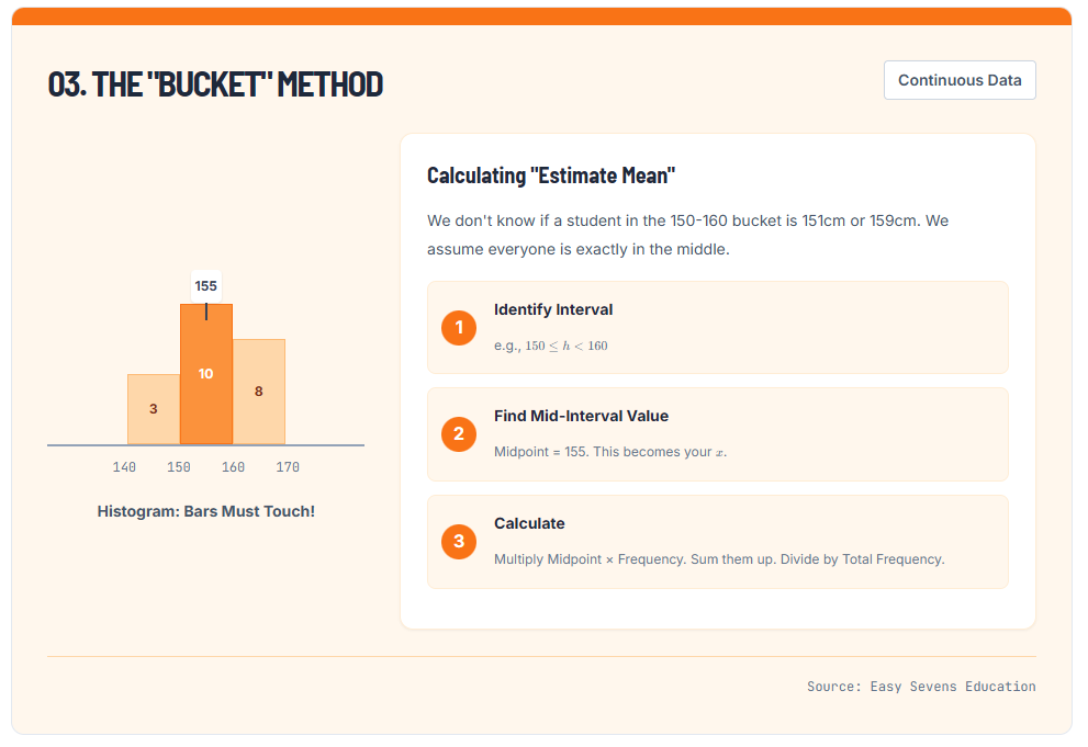
When dealing with continuous data, we often don’t have the raw numbers. Instead, we have “buckets” or class intervals. For example:
- 140 \le h < 150 (Frequency: 3)
- 150 \le h < 160 (Frequency: 10)
If a question asks you to “Calculate the Mean,” and you only have these intervals, you cannot find the true mean because you don’t know if the students in the 150-160 bucket are 151cm or 159cm.
03. The "Bucket" Method
Calculating "Estimate Mean"
We don't know if a student in the 150-160 bucket is 151cm or 159cm. We assume everyone is exactly in the middle.
The Solution: Mid-Interval Values
To estimate the mean, we assume every data point in the bucket is exactly in the middle.
- Find the midpoint of the interval. (e.g., for 140-150, the midpoint is 145).
- Multiply this midpoint by the frequency.
- Sum these products and divide by the total frequency.
Note: Always write “Estimate Mean” in your workings to show you understand the limitation of the data.
The Calculator Hack: TI-Nspire Menu 4.1.1
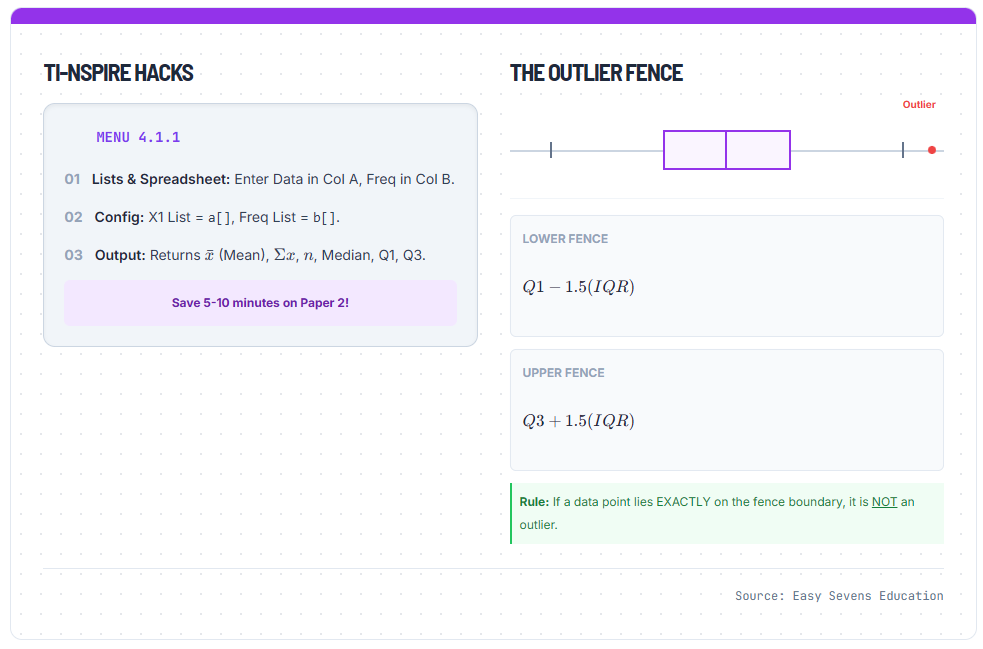
In Paper 2 (and Paper 3 for HL), efficiency is key. You should not be calculating means of large frequency tables by hand. The TI-Nspire has a built-in function for this: One-Variable Statistics.
TI-Nspire Hacks
- 01Lists & Spreadsheet: Enter Data in Col A, Freq in Col B.
- 02Config: X1 List =
a[], Freq List =b[]. - 03Output: Returns \( \bar{x} \) (Mean), \( \Sigma x \), \( n \), Median, Q1, Q3.
The Outlier Fence
Lower Fence
\( Q1 - 1.5(IQR) \)
Upper Fence
\( Q3 + 1.5(IQR) \)
Step-by-Step Guide
- Open a Spreadsheet: Press
Home>Lists & Spreadsheet. - Label Your Columns:
- Label Column A as
data(or specific name likescore). - Label Column B as
freq(if you have a frequency table).
- Label Column A as
- Enter Data: Input your values in Column A and corresponding frequencies in Column B. (If you have raw data lists without frequencies, just use Column A).
- The Magic Command:
- Press
Menu. - Select 4: Statistics.
- Select 1: Stat Calculations.
- Select 1: One-Variable Statistics.
- Press
- Configure the Box:
- Num of Lists: 1.
- X1 List: Type
a[](or select your variable name). - Frequency List: Type
b[](or select your frequency variable). Note: If you don’t have frequencies, leave this as 1. - Result Column: Choose an empty column (e.g., C or D) so you don’t overwrite your data.
Interpreting the Results:
- \bar{x}: This is your Mean.
- \sum x: The sum of all data points.
- n: Total number of data points (Check this to ensure you didn’t miss any values!).
- MedianX: Your Median.
- Q1 / Q3: Your Quartiles (essential for Box and Whisker plots).
Related Resources
Understanding central tendency is just the first step in mastering IB Statistics. Once you can find the center of the data, the next logical step is to analyze how spread out the data is using quartiles and identifying outliers.
For more study guides and math resources, check out our other articles:
Conclusion
Mastering the measures of central tendency is about more than just punching numbers into a calculator. It requires identifying the nature of your data (discrete vs. continuous) and applying the correct logic to find the true center. Whether you are averaging two median positions for an even dataset or using the midpoint method for grouped data, precision is key.
Remember, the IB examiners love to test your understanding of these definitions, not just your ability to do arithmetic. Use the Menu 4.1.1 hack on your TI-Nspire to handle the heavy lifting, but keep your logical brain engaged to interpret the results correctly.
Need help clarifying these concepts or preparing for your next Crit A assessment? Contact Easy Sevens Education today for IB Math guidance on navigating the IB Math curriculum.
Frequently Asked Questions (FAQ)
What do I do if my data has two modes?
If two values appear with the equal highest frequency, the dataset is “bimodal.” You should list both values as the mode. If three or more tie, it is multimodal.
Can I calculate the mean of a histogram?
When should I use Median instead of Mean?
How do I find the median if n=50 without writing it out?
Use the even number rule: Find the value at position 25 (n/2) and position 26 (n/2 + 1). Add those two values together and divide by 2.
Is height discrete or continuous?
Height is continuous. Even though we might say “170 cm,” in reality, height can be measured to infinite decimal places given a precise enough tool. Therefore, we treat it as continuous data in histograms.